Predicting House Prices in Ames, Iowa

This project predicts home sale prices using linear (ElasticNet) and non-linear (XGBoost) regression models trained on over 80 features. It incorporates robust preprocessing, feature engineering, and model tuning to achieve strong predictive accuracy.

The Dataset and the Goal

The data is the Ames Housing dataset, a record of roughly 2,900 residential sales in Ames, Iowa between 2006 and 2010. Each home is described by more than 80 features covering size, quality, location, and condition, ranging from square footage and year built to neighborhood, basement finish type, and kitchen quality. It is a well-known alternative to the older Boston housing data, and its appeal is that the features are messy in realistic ways: a mix of numeric, ordinal, and high-cardinality categorical columns, missing values that carry meaning rather than noise, and a handful of unusually large properties that distort any model fit with squared error.

The goal was to predict sale price from those features, and to do it with two different model families so the results could be compared: one regularized linear model and one gradient-boosted tree model. Performance was measured as RMSE between the natural logarithm of the predicted and actual sale price, evaluated across ten predefined train/test splits. Working in log space means the model is penalized for proportional error rather than absolute dollars, so missing on a $500,000 home by 10% costs the same as missing on a $100,000 home by 10%. Each split came with a fixed accuracy threshold that both models had to clear, 0.125 RMSE for the first five and 0.135 for the last five.

Data Exploration

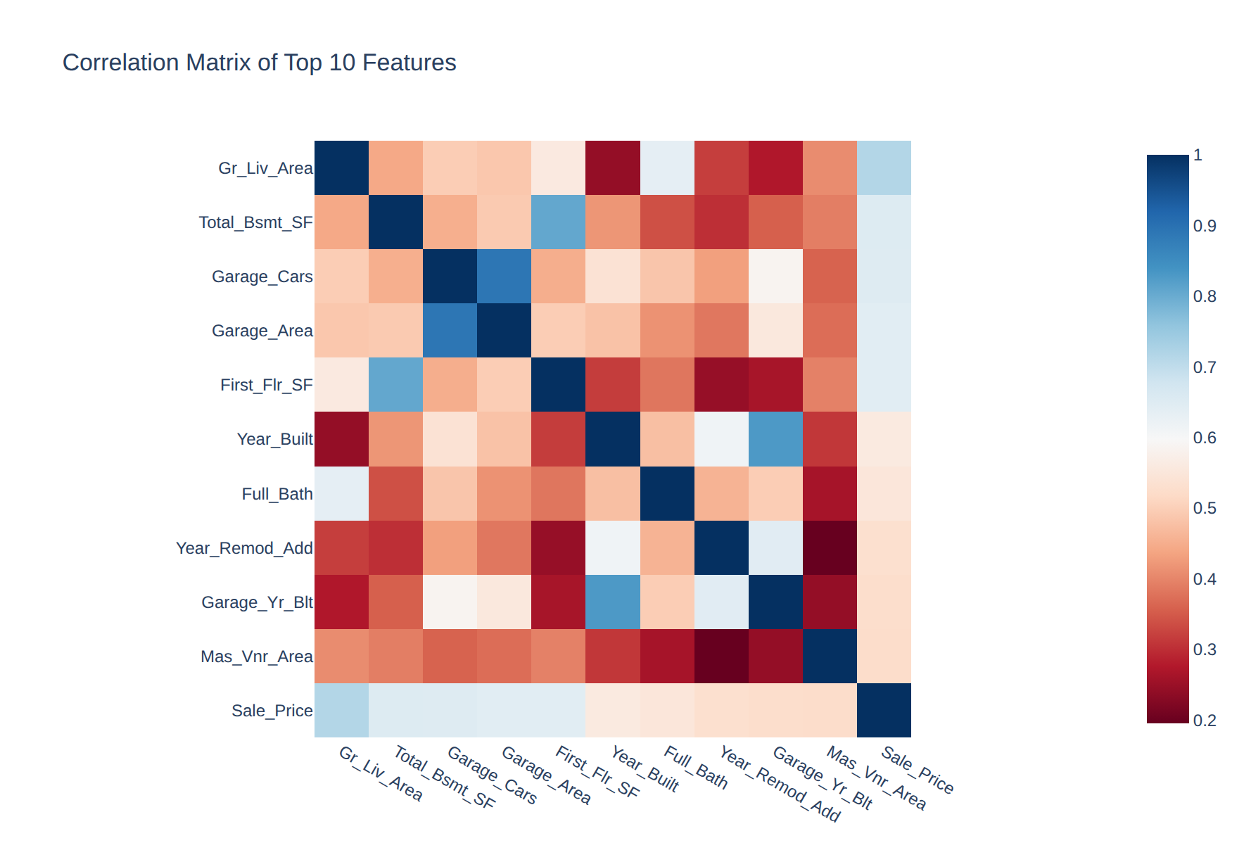
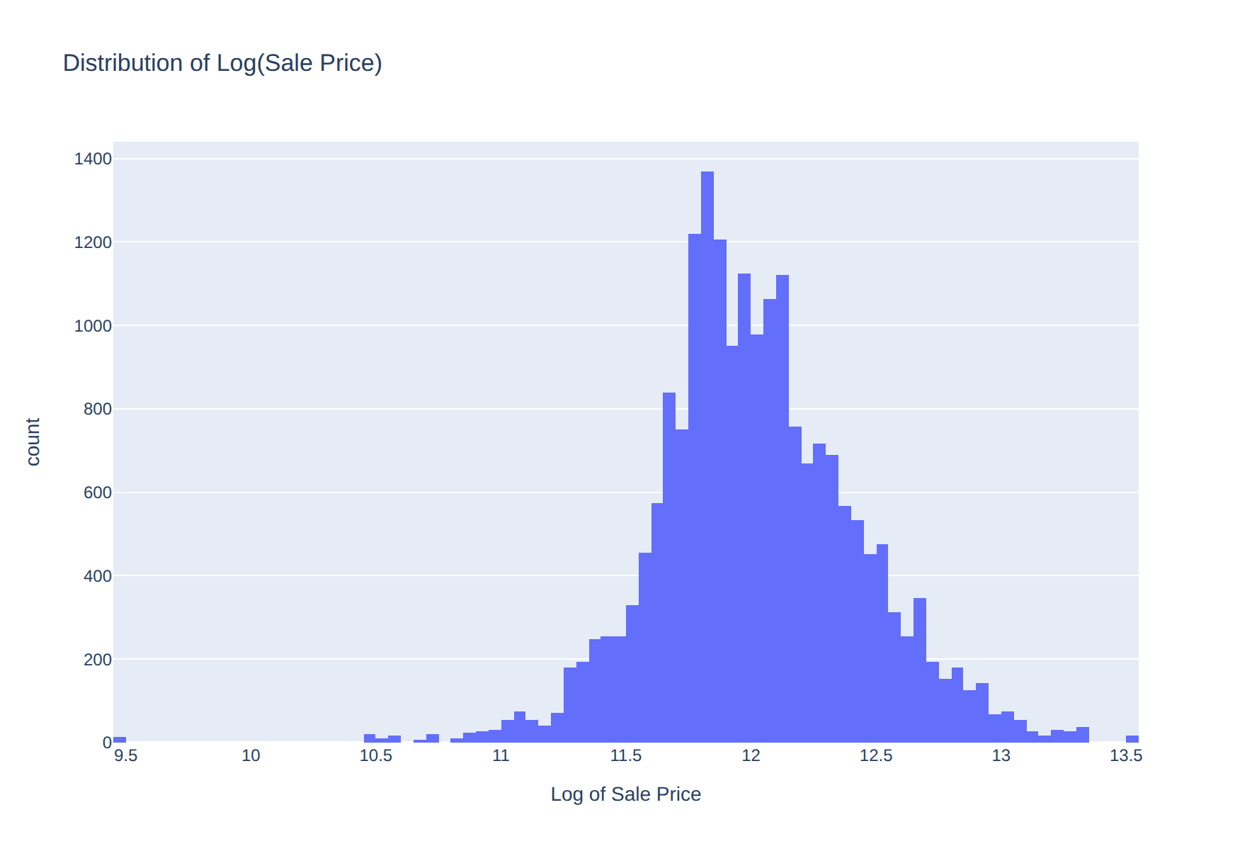
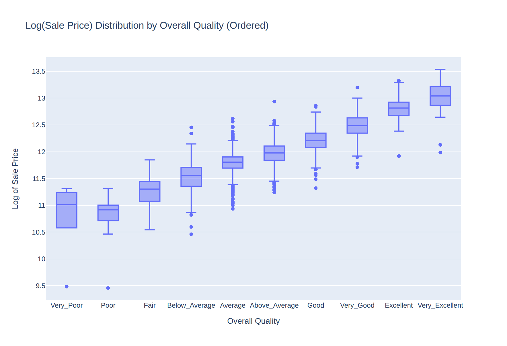
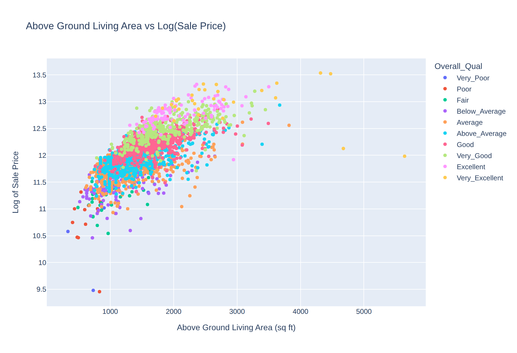
I began by exploring the relationship between predictors and the response (home sale prices) to guide feature transformations and model selection. To get a feel for the data, I examined scatter plots, counted null values, and examined distributions of categorical and numerical variables. The interactive charts below highlight some of the more apparent patterns, such as the strong log-linear relationship between living area and sale price, and the ordinal impact of overall quality.

Data Preprocessing

• Removed 11 low-utility columns. These were either redundant or mostly null values.
• Filled missing values in Garage_Yr_Blt with 0 to preserve numeric format.
• Winsorized 15+ numerical features at the 95th percentile to reduce outlier influence.
• Identified categorical features and applied full one-hot encoding (K dummies per column, no level dropping).
• Standardized numerical features using RobustScaler for stability against outliers.
• Log-transformed Sale_Price to normalize its distribution and align with RMSE evaluation.

Model Tuning

• For ElasticNet, performed a grid search on alpha and l1_ratio based on initial exploration, then used ElasticNetCV for cross-validation.
• Applied RobustScaler to inputs before fitting the linear model.
• For XGBoost, used parameters inspired by community benchmarks: n_estimators=5000, max_depth=6, eta=0.01, and subsample=0.5.
• XGBoost performed well without further tuning due to the robustness of tree-based methods to raw feature scale.

Evaluation

• Used Root Mean Squared Error (RMSE) on the natural log of sale price for all model evaluations.
• Validated both models using 10 distinct train/test splits, reporting scores separately for each fold.
• Both models were below 0.125 RMSE for the first 5 folds and below 0.135 for last 5.
• XGBoost consistently outperformed ElasticNet, capturing non-linear relationships in the data.

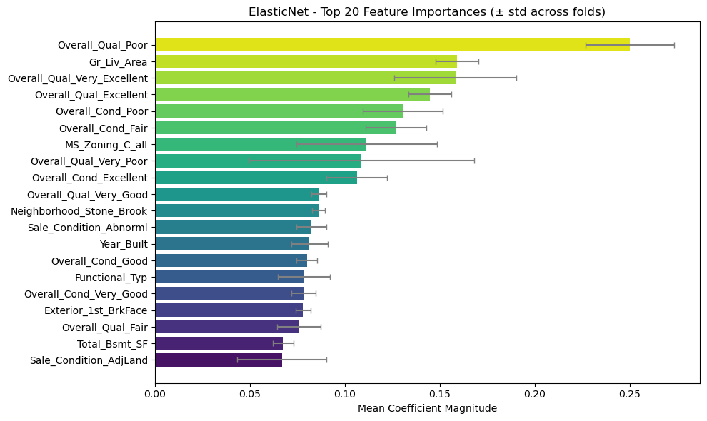
Figure: Top ElasticNet Features

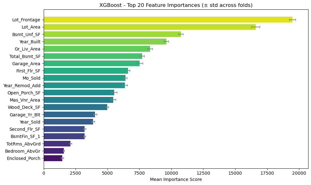
Figure: Top XGBoost Features

Above are the most influential features for each model, aggregated across all folds. The linear ElasticNet model strongly emphasizes features we identified early in our data exploration, particularly living area and overall quality. In contrast, XGBoost appears to deprioritize the Overall_Qual categories entirely. Interestingly, only three features appear in the top 20 for both models: Year_Built, Gr_Liv_Area, and Total_Bsmt_SF. This aligns with our intuition that these features are key predictors of sale price, but also highlights the different ways linear and non-linear models can interpret feature importance.