
Weekly sales for 45 Walmart stores from 2010 to 2012, with a benchmark WMAE of 1580 to beat. The metric weights the four big holiday weeks five times heavier than everything else, so the whole problem is really about not being wrong at Christmas.
I started with the dumbest thing that could work: look up what the same store and department sold this week last year. That got 1888. What follows is finding out which of my ideas actually beat that, and which ones only felt clever.
Dataset & Evaluation Metric
This project is based on the Walmart Store Sales Forecasting competition dataset. The data contains historical weekly sales from February 2010 to October 2012 for 45 stores across various departments.
The primary success metric was Weighted Mean Absolute Error (WMAE), where four key holidays—Super Bowl, Labor Day, Thanksgiving, and Christmas—are weighted five times higher than regular weeks. This metric emphasizes the business-critical need for accurate holiday predictions. To ensure robust evaluation, I used 10 time-based cross-validation folds, training on a growing window of historical data and forecasting the subsequent two months.
Initial Data Exploration
I began by visualizing the sales patterns across several key departments. The chart below immediately highlighted the complexity of the problem. Some departments exhibited smooth, predictable seasonality, while others had sharp holiday spikes or erratic trends. This initial insight motivated my decision to use department-specific modeling and calendar-aware features from the very beginning.
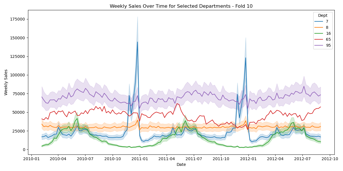
Figure: Weekly Sales Over Time for Departments 7, 8, 16, 65, and 95
The Model Evolution: A Step-by-Step Journey
My approach was iterative. I started with the simplest possible models to establish a baseline and systematically added complexity, measuring the impact of each decision on the WMAE.
Step 1: Establishing a Baseline
First, I needed a starting point. As shown in my exploratory notebook, I implemented a naive model that simply used the last known sales figure for each store-department pair. This gave me a WMAE of ~2078. A slightly better seasonal model, which matched sales to the same week from the previous year, improved this to 1888. These initial results proved that simple lookups were insufficient and a more robust modeling approach was necessary.
WMAE: 1888
Step 2: Introducing Time-Based Regression
My next step was to build a proper regression model. I developed a function, preprocess, to engineer features from the 'Date' column, creating Yr, Yr2, and Wk variables to capture trends and seasonality. Using patsy and statsmodels, I fit an Ordinary Least Squares (OLS) model for each store-department combination. This more structured approach significantly lowered the error.
WMAE: 1658 → 1626
Step 3: SVD Denoising
While the regression model was an improvement, its predictions were still noisy. I hypothesized that many sales figures were driven by random fluctuations rather than true signals. To address this, I implemented a denoising step using Singular Value Decomposition (SVD) in my svd_dept function.
- For each department, I created a Store × Date matrix of sales data.
- I then applied
np.linalg.svdto decompose this matrix, isolating the principal components of the sales data. - By reconstructing the matrix using only the top 8 singular components, I effectively filtered out the noise while retaining the core sales patterns.
This took WMAE from 1626 to 1588, which put the model within 8 points of the benchmark.
WMAE: 1588
Step 4: A Final Polish with Holiday Smoothing
The final challenge was the holiday season (weeks 49-52), where the WMAE metric was 5x more sensitive. My SVD-enhanced model was still over-predicting sharp, brief spikes. To create a more realistic forecast, I wrote a post-processing function called apply_shift. For holiday weeks, this function adjusted the prediction by blending it with the previous week's sales (85% current prediction + 15% previous week's prediction). This small, domain-aware adjustment smoothed the volatile holiday peaks and provided the final improvement needed to beat the benchmark.
WMAE: 1559.5
Validating the Granular Approach with Cluster Analysis
To further confirm my hypothesis that a single, global model would fail, I performed cluster analysis on the sales data, grouping both stores and departments by their standardized weekly sales curves. The results, shown below, were definitive.
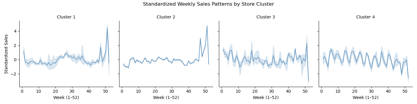
Figure: Standardized Weekly Sales by Store Cluster (Agglomerative, k=4)
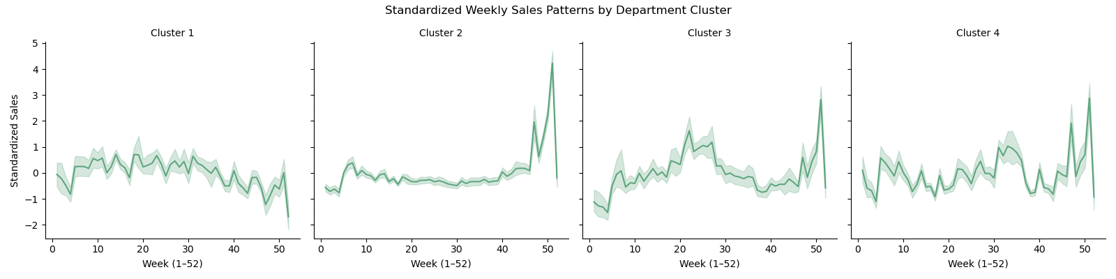
Figure: Standardized Weekly Sales by Department Cluster (Agglomerative, k=4)
The analysis revealed distinct groups with vastly different seasonal cycles, volatility, and overall sales patterns. This data-driven insight validated my core architectural decision: to build a separate, fine-tuned model for each individual store-department pair rather than attempting a one-size-fits-all solution.
What did not work
Three things are worth saying, because the numbers above only go one direction and that is not what the work felt like.
- The seasonal baseline was a dead end, not a foundation. Matching each store-department to the same week last year got 1888, and no amount of tuning that idea was going to get near 1580. It was useful for telling me the naive answer was not close, and that is all it was useful for.
- Regression did most of the work, but it did not feel that way. Going from the baseline to a proper OLS model per store-department bought 1658, then 1626, the biggest drop on this page. It still left me well short of 1580, and at that point I was not confident the approach was going anywhere.
- Denoising made the holidays worse before it made them better. SVD cleaned up the general signal and got to 1588, but it left the model over-predicting sharp holiday spikes, which is exactly where the metric punishes you five times harder. The blend in step 4 exists because the step before it introduced that problem, not because I planned it.
Final Results and Conclusion
The final pipeline averaged a WMAE of 1559.5 against a benchmark of 1580, so it cleared it by about 1%. That is a real result and it is also a narrow one, which is the honest way to describe it. What I would take from this project is less about OLS or SVD and more about the fact that the last step, a two-line weighted blend in the holiday weeks, moved the number as much as the fancy matrix decomposition did. Knowing the metric weights Christmas five times heavier was worth more than any modelling technique I applied.
Final Average WMAE:
1559.5
Benchmark to Beat: 1580